Credit Risk Modelling
Problem description
LendingClub’s complete loan data issued from 2007-2017 was used to build LGD, EAD, and PD models.
Calculating LGD
Loss given Defaults(LGD): The proportion of the total exposure that cannot be recovered by the lender once a default has occured
LGD = 1 - Recovery Rate
first the recovery rate is calculated dividing the amount recovered by the total amount
loan_data_defaults['recovery_rate'] = loan_data_defaults['recoveries'] / loan_data_defaults['funded_amnt']
table will look like this
| id | funded_amnt | recoveries | recovery_rate |
|---|---|---|---|
| 0 | 112435993 | 0 | 0 |
where funded_amt is total amount loaned to customer and recoveries is the amount recovered.
Then the LGD can be calculated as such
loan_data_defaults['LGD'] = 1- loan_data_defaults['recovery_rate']
| id | funded_amnt | recoveries | recovery_rate | LGD |
|---|---|---|---|---|
| 0 | 112435993 | 0 | 0 | 0 |
Calculating EAD
Exposure at Default(EAD): The total value that a lender is exposed to when a borrower default
important for calculating regulatory capital requirements.
helps lenders assess their risk appetite and allocate capital accordingly.
EAD can be calculated as such
EAD = total funded amount (drawn + undrawn) x credit conversation factor
But first the credit conversation factor is calculated. It is the ratio of the difference of the amount used at the moment of default to the total funded amount.
loan_data_defaults['CCF'] = (loan_data_defaults['funded_amnt'] - loan_data_defaults['total_rec_prncp']) / loan_data_defaults['funded_amnt']
where total_rec_prncp reflects the total payments made on the principal of the loan
| id | funded_amnt | recoveries | recovery_rate | LGD | CCF |
|---|---|---|---|---|---|
| 0 | 2300 | 0 | 0 | 0 | 0.88 |
loan_data_defaults['EAD'] = loan_data_defaults['funded_amnt'] * loan_data_defaults['CCF']
| id | funded_amnt | recoveries | recovery_rate | LGD | CCF | EAD |
|---|---|---|---|---|---|---|
| 0 | 2300 | 0 | 0 | 0 | 0.88 | 2029 |
PD modelling
Logistic regression was used to calculate the PD
The ‘LogisticRegression’ class from the sci-kit learn package was used to calculate the PD’s
Below is the summary table showing the feature name, coefficients, and p-values for the PD model. A total of 83 features were used to create the model but the table below shows only 3 of those features.
| Feature name | coefficients | p-values |
|---|---|---|
| home_ownership:OWN | 0.122694 | 2.786529e-01 |
| home_ownership:MORTGAGE | 0.124868 | 5.696552e-75 |
| emp_length:1 | 0.079714 | 6.910273e-02 |
The training population was labeled 1 where loan status = default, else labeled 0.
df['loan_status'].unique()

# Output, the different types of labels showing the status of the loan

array(['Fully Paid', 'Charged Off', 'Current', 'In Grace Period',
       'Late (31-120 days)', 'Late (16-30 days)', 'Default',
       'Does not meet the credit policy. Status:Fully Paid',
       'Does not meet the credit policy. Status:Charged Off'],
      dtype=object)
A pd value was calculated for each observation in the test population.
where every observation that has predicted probability greater than the threshold has a value of 1, and every observation that has predicted probability lower than the threshold has a value of 0.
the threshold is set at 0.9
The below table shows the confustion matrix, where the actual values are displayed by rows and the predicted values by columns.
| Predicted | 0 | 1 |
|---|---|---|
| Actual | ||
| 0 | 7408 | 2782 |
| 1 | 36747 | 46320 |
The Receiver Operating Characteristic (ROC) curve was created using the code below.
fpr, tpr, thresholds = roc_curve(df_actual_predicted_probs['loan_data_targets_test'], df_actual_predicted_probs['y_hat_test_proba'])
# Here we store each of the three arrays in a separate variable.

plt.plot(fpr, tpr)
# We plot the false positive rate along the x-axis and the true positive rate along the y-axis,
# thus plotting the ROC curve.
plt.plot(fpr, fpr, linestyle = '--', color = 'k')
# We plot a seconary diagonal line, with dashed line style and black color.
plt.xlabel('False positive rate')
# We name the x-axis "False positive rate".
plt.ylabel('True positive rate')
# We name the x-axis "True positive rate".
plt.title('ROC curve')
# We name the graph "ROC curve".
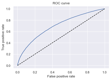
The gini was then calculated from the Area Under the Receiver Operating Characteristic Curve (AUROC) as such
AUROC = roc_auc_score(df_actual_predicted_probs['loan_data_targets_test'], df_actual_predicted_probs['y_hat_test_proba'])
# Calculates the Area Under the Receiver Operating Characteristic Curve (AUROC)
# from a set of actual values and their predicted probabilities.

Gini = AUROC * 2 - 1
# Here we calculate Gini from AUROC.
The gini equals 0.40