Customer Segmentation

Problem description

Ecommerce companies usually cluster and segment customers, this is in order to preform cohort analysis. For example, personalising emails.

understanding the data

import pandas as pd
import numpy as np
import matplotlib.pyplot as plt
import seaborn as sns
from sklearn.cluster import KMeans
from sklearn.metrics import silhouette_score
from sklearn.preprocessing import StandardScaler

df= pd.read_csv('Mall_Customers.csv')
df.head()

CustomerID	Gender	Age	Annual Income (k$)	Spending Score (1-100)
1	Male	19	15	39

Unique ID assigned to the customer

Gender:Gender of the customer

Age:Age of the customer

Annual Income (k$): Annual Income of the customer

Spending Score (1-100):Score assigned by the mall based on customer behavior and spending nature

Assuming the higher the spending score, the more a customer spends per purchase

Conducting EDA

col_names = ['Annual Income (k$)', 'Age', 'Spending Score (1-100)']
df.hist(col_names)

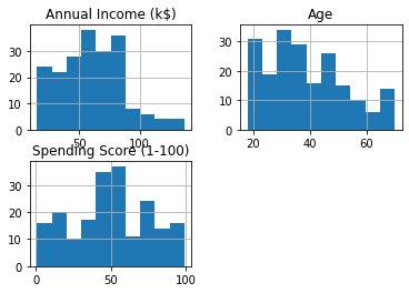
numbers excluding customer id are on different scales therefore must standardise. customer id can be dropped

Pre-processing

features = df[col_names]
scaler = StandardScaler().fit(features.values)
features = scaler.transform(features.values)
scaled_features = pd.DataFrame(features, columns = col_names)

Gender is catagorical , we must encoding into a numerical data type

Hyperparameter tunning

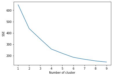
Elbow method

sse = {}
for k in range(1, 10):
    kmeans = KMeans(n_clusters=k, max_iter=1000).fit(newdf)
    newdf["clusters"] = kmeans.labels_
  
    sse[k] = kmeans.inertia_ # Inertia: Sum of distances of samples to their closest cluster center
plt.figure()
plt.plot(list(sse.keys()), list(sse.values()))
plt.xlabel("Number of cluster")
plt.ylabel("SSE")
plt.show()

• For each value of k:
  • For each cluster c:
    • calculate the within cluster sum of squared distances
    • the distance between each point in cluster and centroid
  • sum the distance values for each cluster

• plot a line graph of the SSE for each value of k.

• SSE tends to decrease toward 0 as we increase k
  • SSE is 0 when k is equal to the number of data points in the dataset
    • because then each data point is its own cluster
    • there is no error between it and the center of its cluster
• Goal is to choose the smallest value of k that has a low SSE,
• The elbow usually represents this part
  • k= 4

Model evaluation

Silhouette Score

kmeans = KMeans( n_clusters = 4, init='k-means++')
kmeans.fit(newdf)

newdf['clusters']= kmeans.fit_predict(newdf)
print(silhouette_score(newdf, newdf['clusters'], metric='euclidean'))
# score: 0.27541910197758873

• Metric used to evaluate the quality of clusters created by the algorithm.

• Silhouette scores range from -1 to +1.

• Mean distance between the observation and all other data points in the same cluster. This distance can also be called a mean intra-cluster distance.

• Mean distance between the observation and all other data points of the next nearest cluster. This distance can also be called a mean nearest-cluster distance.

• A good clustering algorithm will
  • minimise the mean intra-cluster distance
  • maximise the mean nearest-cluster distance

• If the score is 1, the cluster is dense and well-separated than other clusters.

• A value near 0 represents overlapping clusters with samples very close to the decision boundary of the neighboring clusters.

• A negative score indicates that the samples might have got assigned to the wrong clusters.

Customer analysis

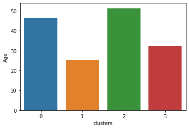
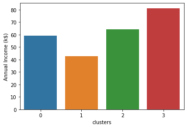
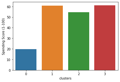
Cluster 0 : intermediate annual income, intermediate spending score

• Early 40s
• 55k annual income
• Intermediate spending score of 49
• Predominantly female

Cluster 1: High annual income, low spending score

• Late 30s
• 86k annual income
• Low spending score of 17
• More or less equal in gender

Cluster 2: High annual income, high spending score

• Early 30s
• 85k annual income
• High spending score of 82
• Predominantly female

Cluster 3: Low annual income, low spending score

• Mid 40s
• 26k annual income
• Low spending score of 21
• Predominantly female

Cluster 4 (yellow): Low annual income, high spending score

• Mid 20s
• 26k annual income
• High spending score of 78
• Predominantly female