Fraud detection

Understanding the data

df = pd.read_csv('creditcard.csv')
df.head()

Time	Amount	class	v1	v28
1.0	149.62	0	-1.359807	-0.021053

• NOTE There are 28 ‘v’ features : v1,…,v28
• Due to privacy reasons most colums dont have a column name
• Time : not enough information about this feature, going to remove
• amount : the monentary amount of the transaction that was flagged as fraud
• classes :
  • 0: No fraud
  • 1: Fraud

Exploratory Analysis (EDA)

plt.bar(x=[0,1],height=[df['Class'].value_counts()[0],df['Class'].value_counts()[1]])

plt.title('Class Distributions (0:No Fraud 1: Fraud)', fontsize=14)

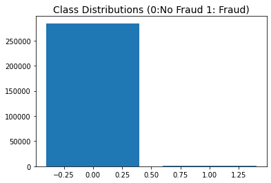
Class
0	284315
1	492

amount_val = df['Amount'].values

fig,ax = plt.subplots()

sns.distplot(amount_val, color='r',ax=ax)
ax.set(title='Distribution of Transaction Amount')
ax.set_xlim([min(amount_val), max(amount_val)])
plt.show()

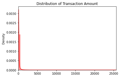
• Tansactions are mainly of smaller amounts

Metric Selection

• very imbalanced class distribution, positive class is minority
• positive class more important than negative class, need to detect if fraud occurs with high confidence
  • e.g. 90% precision
• False negatives; falsely classifiying fraud sample as not fraud is very costly need to minimise.
  • need as low as possible
  • trade-off: high recall as possible due to False negatives
    • but precision needs to be above a threshold to be useful
• Precision, recall,f1 measure and False negatives going to be used to compare models via cv

Pre-processing

• Dataset was scaled, used robust scaler which is more robust to outliers
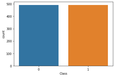
• To better visualise the data and conduct multi-vartiate analysis, will implement a random under sampling technique, which undersamples the majority class, creating a more balanced dataset

rob_scaler = RobustScaler()

X = df.drop(['Class','Time'],axis=1)
y = df['Class']

X_scaled = rob_scaler.fit_transform(X)

X_scaled_df = pd.DataFrame(X_scaled, columns = X.columns)

rus = RandomUnderSampler(random_state=42)

X, y = rus.fit_resample(X, y)

sns.countplot(y)

balanced_df = pd.DataFrame(X.join(y))

corr = balanced_df.corr()
sns.heatmap(corr, cmap='coolwarm_r', annot_kws={'size':20}).set_title("Imbalanced Correlation Matrix", fontsize=14)

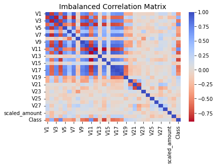
• v4, v11 features are highly positively correlated with class
• v14 andv10 are highly negatively skewed with class
• no features are hightly correlated with eachother
  • if there was highly correlated features , should remove

Model selection

• Needed to split the data into training and test sets, then apply transformation in pipeline
  • to prevent leakage when estimating model preformance on via cross-validation.
  • Used stratified random sampling, as dataset very imbalanced
• reloaded orginal unbalanced dataset

X = df.drop(['Class','Time'],axis=1)
y= df['Class']
X_train, X_test, y_train, y_test = train_test_split(X,y,stratify=y,random_state=1)

Baseline score, without resampling or specialised imbalanced algorithms

• First going to use:
  1. naive model: dummy classifier which outputs uniform results
  2. logistic regression
  3. random forest
  4. neural network
• Aim: get a baseline score without specialised algorithms designed for imbalanced learning
  • naive algorithms without resampling etc
• The first 3 models were implemented using the sci-kitlearn library
  • stratified 10 fold cv was used to calculate f1, precision and recall values
• The neural network model was implemented using the tensorflow library

sci-kit learn (model 1,2 and 3)

from sklearn.dummy import DummyClassifier
from sklearn.pipeline import Pipeline

pipe1 = Pipeline([
    ('scaler',RobustScaler()),
    ('model',DummyClassifier(strategy='uniform'))
])

pipe2 = Pipeline([
    ('scaler',RobustScaler()),
    ('model',LogisticRegression())
])

pipe3 = Pipeline([
    ('scaler',RobustScaler()),
    ('model',RandomForestClassifier())
])

from sklearn.model_selection import cross_validate
from sklearn.model_selection import StratifiedKFold

cv = StratifiedKFold(n_splits=10)
scores= ['f1','precision','recall']

navie_cv_results = cross_validate(pipe1,X=X_train,y=y_train,cv=cv,scoring=scores,n_jobs=-1)
logistic_cv_results = cross_validate(pipe2,X=X_train,y=y_train,cv=cv,scoring=scores,n_jobs=-1)
randomForest_cv_results = cross_validate(pipe3,X=X_train,y=y_train,cv=cv,scoring=scores,n_jobs=-1)

The mean f1, precision and recall scores

model_1: naive algo

	0
test_f1	0.00347783
test_precision	0.00174494
test_recall	0.503979

model_2: logistic regression

	0
test_f1	0.685409
test_precision	0.852982
test_recall	0.577477

model_3: random forest

	0
test_f1	0.840989
test_precision	0.948857
test_recall	0.756156

• clearly the naive algo performs the worst
• mean scores from cv does not show the whole picture
  • must visualise learning curves to diagnose any problems in the learning stage

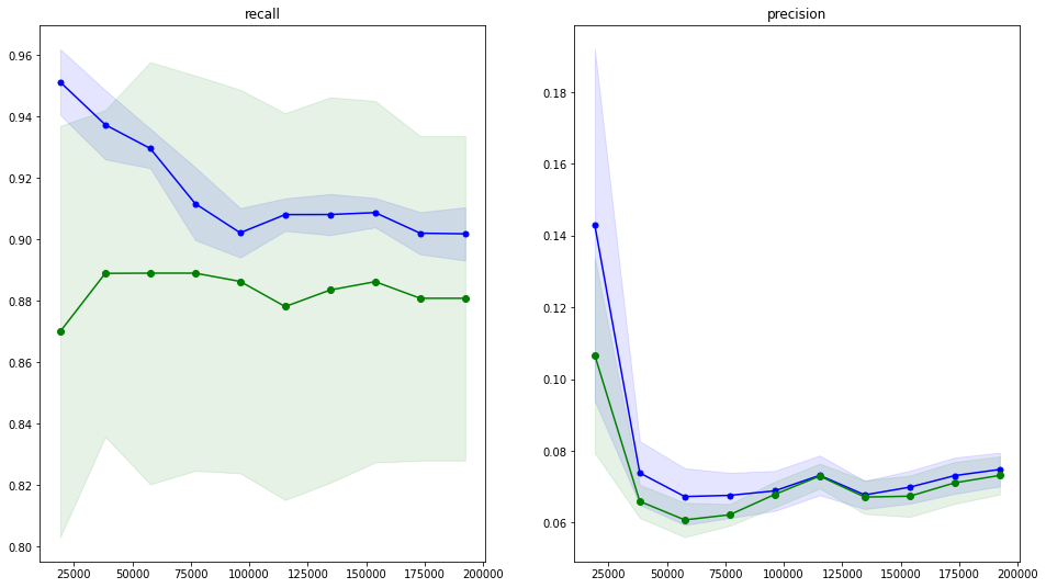
The precision and recall learning curves

model_2: logistic regression

• logistic regression seems to be the best, but recall score is low

model_3: random forest

• randomforest is overfitting
  • represented by large gap between the training and test scores

Tensorflow neural network

• The neural network will be built via a different library called keras

METRICS = [
  keras.metrics.Precision
  keras.metrics.FalseNegatives
  keras.metrics.Recall
]

def make_model(metrics=METRICS, output_bias=None):
  if output_bias is not None:
    output_bias = tf.keras.initializers.Constant(output_bias)
  model = keras.Sequential([
      keras.layers.Dense(
          16, activation='relu',
          input_shape=(train_features.shape[-1],)),
      keras.layers.Dropout(0.5),
      keras.layers.Dense(1, activation='sigmoid',
                         bias_initializer=output_bias),
  ])

  model.compile(
      optimizer=keras.optimizers.Adam(learning_rate=1e-3),
      loss=keras.losses.BinaryCrossentropy(),
      metrics=metrics)
  
  return model 

  model.compile(
      optimizer=keras.optimizers.Adam(learning_rate=1e-3),
      loss=keras.losses.BinaryCrossentropy(),
      metrics=metrics)
  
  return model 

EPOCHS = 100
BATCH_SIZE = 2048

early_stopping = tf.keras.callbacks.EarlyStopping(
    monitor='val_prc', 
    verbose=1,
    patience=10,
    mode='max',
    restore_best_weights=True)

model = make_model()
model.summary()

type	Output Shape	Param
Dense	(None, 16)	480
Dropout	(None, 16)	0
Dense	(None, 1)	17

• Total params: 497
• Trainable params: 497
• Non-trainable params: 0

concluding first stage

• logistic regression and Random Forest is shortlisted
  • the complexity of the algorithms will be increased

Specialised algorithms

• Implemented SMOTE and cost-sensitive learning on the shortlisted model

• logic of using cv for imbalanced learning:

  • up/down sampling done in inside cv
  • imblearn.pipeline extends scikit-learn pipeline.
  1. Up/downsampled only the data in the training section
  2. Fit the model on the up/down sampled training data
  3. Score the model on the (non-up/downsampled) validation data

recall/precision trade-off

• SMOTE and balanced class wieghts increases recall at the cost of precision

from imblearn.pipeline import Pipeline as imbpipeline
pipeline1 = imbpipeline([
    ['smote', SMOTE(random_state=11)],
    ['scaler',RobustScaler()],
    ['classifier', LogisticRegression(random_state=11,penalty='l2', n_jobs=-1, max_iter=1000)]
    ])

• precision of ~0.03 is not acceptable