Trading System
Problem Description
The aim for this project was to develop an end-to-end machine learning (ML) system; to better understand ML system design. A vital skill for ML engineers. Initially the scale and scope of the project was small, however as time progressed the complexity and size grew. And with that growth in complexity, I had to learn new skills to keep up with the technical demand.
Skills learnt: docker, Amazon Web services (ECS, S3), DevOps practices, Java, Kafka, Redis
Skills developed: time series analysis and feature construction, feature selection
Data architecture hosted on AWS on a high availability cluster ECS:
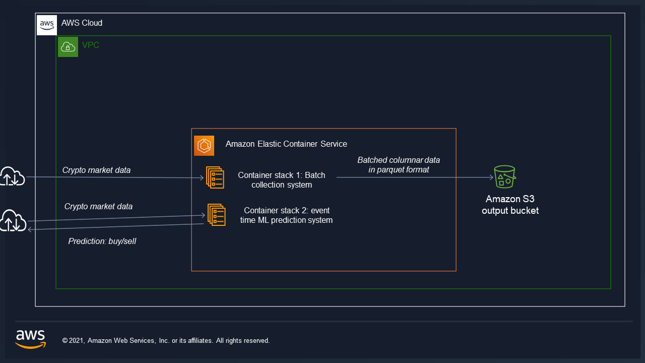
Task
The task was to utilise data science techniques to gain insights from financial time series data, and ultimately to build ML learning models to exploit those insights and predictive trading signals in buy or sell a particular crypto-currency pair.
The reason I focused on the cryptocurrency market is because tick and orderbook data for traditional financial instruments is expensive. Whereas most crypto exchanges allow access to market feed via API.
Two data pipelines are containerised. one to collect for offline data analysis and ML and the other low latency system to predict trading signals via online ML.
Data Collection
Market data was collected from 15 cryptocurrency exchanges, I forked a open-source project which handles the data feeds for most exchanges called cryptofeed https://github.com/bmoscon/cryptofeed
building ontop of the code and using to existing redis backend to batch the data every one minute (proccess time) and save as parquet files to my private s3 bucket using the aws api.
example tick data from BTC_USDT pair [figure1]
| index | price | volume | signed_tick |
|---|---|---|---|
| 2021-02-01 00:00:00.235000 | 33084.6 | 0.060084 | -1 |
example l2 orderbook data from BTC_USDT pair [figure2]
| timestamp | receipt_timestamp | delta | side | price | size |
|---|---|---|---|---|---|
| 2021-10-20 14:09:55.026000128 | 2021-10-20 14:12:25.604629504 | True | bid | 65961.2 | 0.00042 |
For the l2 data the pipeline is configured to take a snapshot of the orderbook for the first 100 levels once every day after midnight The rest of the updates are changes made to the orginal snapshot.
Time series analysis
Non independently identically distributed (IID) Financial data
The algorithms and techniques used were from Lopez de Prado (2018).
A sampling technique was used to construct ‘information-driven bars’, to idea is to sample more frequently from the tick feed as shown on figure1. When new information arrives to the market a information bar is conducted, which represents one row. The columns are the same as normal time-based bar features : open, high, low and close.
example information-driven as explained by Lopez de Prado (2018) [figure3]
| date_time | open | high | low | close |
|---|---|---|---|---|
| 2021-02-03 00:00:00.134000 | 1511.93 | 1512.11 | 1511.93 | 1512.11 |
This data set can be thought of as the main data set used to construct other features or enrich with supplementory orderbook data.
The reason for sampling when new information arrives is because financial time series is not independently identically distributed (IID). Machine learning models assume the data is IID. Sampling This way is to ensure the data is more IID.
Stationarity and memory trade-off
To build a ML model to make predictions based on historical financial time series the data must be made stationary. As supervised learning models require stationary features. However this reduces the memory of the series. The idea is to fractionally differentiate the price series in order to make the data stationary, but preserve as much memory as possible.
I used the Augmented Dickey-Fuller Test to analyse the stationary and memory trade-off.
The Augmented Dickey-Fuller test is a type of statistical test called a unit root test.
Where :
- Null Hypothesis (H0): If failed to be rejected, it suggests the time series has a unit root, meaning it is non-stationary. It has some time dependent structure.
- Alternate Hypothesis (H1): The null hypothesis is rejected; it suggests the time series does not have a unit root, meaning it is stationary.
The results are interpreted using the p-value method.
p-value > 0.05: Fail to reject the null hypothesis (H0), the data has a unit root and is non-stationary. p-value <= 0.05: Reject the null hypothesis (H0), the data does not have a unit root and is stationary.
from statsmodels.tsa.stattools import adfuller

close_ffd = close.apply(np.log).cumsum().to_frame()

close_ffd =  frac_diff_ffd(series=close_ffd,
                            diff_amt=1.9999981,thresh=0.000001).dropna()

p_val= adfuller(close_ffd,maxlag=1,regression='c',autolag=None)[1]

print(p_val)

#0.04600717533264174
In the code above I log tansformed the close price seris of the data from figure 3, then applied the cumsum transformation. This helps preserve the memory of the data. In example above the p value is below 0.05 therefore the series is stationary.
cumsum filter
Lopez de prado (2018) states event-based sampling should be implemented using a cusum filter, market prices tend to fluctuate during a market event; big sell off, news etc. The cusum filter is designed to detect a shift in the mean of the prices, and market events cause a shift in the mean. The machine learning model will only learn from data where the mean
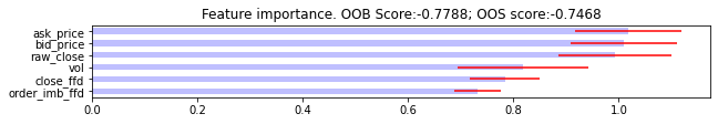
Feature selection
References
Lopez de Prado, M. (2018). Advances in financial machine learning. John Wiley & Sons.